Vulkan Engine
Vertical Slice Game Engine using Vulkan
Created as a way to prove out and learn a number of key engine features, it now exists as a small scale engine usable for simple 3D projects
Content
Introduction
This engine originated through the process of learning Vulkan for the first time. It was originally intended as a simpler project with only a few features to get used to using the newer API. As I continued to learn, the project expanded as I began to use it as the ‘go-to’ 3D rendering project for the subject at hand. This collection of usable game features provides a good baseline for game engines I build in the future and currently remains usable for smaller, simpler 3D projects. Some of these features have been recreated for the new engine I’m building while learning DirectX 12!
Features
The engine contains a series of features (most of which are my first ever implementations) which can be used to develop 3D games. The main ones I will be discussing in this post are:
- Asset Management System
- Vulkan Renderer
- Custom Collision Detection and Response System
- Terrain Generation
Structure
The solution consists of two key parts:
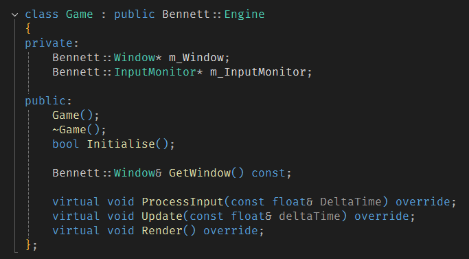
- Engine Project - The core of the engine exists here. All of the building blocks of the rendering, collision, world, physics are written in this project. It compiles as a DLL so that it can be used as a basis for individual game projects.
- Test Game Project - This is the front facing project used as an example scene for various game features. This project utilises the exported engine DLL to create a window, renderer and asset storage system to create the game world.
A standalone editor project was worked on for a small amount of time but it was ultimately scrapped in favour of focussing on additional features over juggling the creation, maintainence and debugging of three projects simultaneously. It was built as an MFC desktop application with the inspiration for the style of the editor coming from classic level editors such as Hammer (Source Engine) and Sapien (Halo).
Asset Management
The asset manager is a publically accessible class that can be retrieved through the service locator. It allows for requests of individual textures and meshes as well as the loading of GLTF files. By loading a GLTF file, the asset manager can load and store references to multiple meshes from a single file such as in the code snippet below. It only loads the file upon the first request as it stores the pointers to the individual meshes themselves using the GLTF hierachy object names as an identifier for an unordered_map. This allows for the quick reuse of assets within a scene as they only utilise a single loaded chunk of data. However, this does reduce the amount of unique names that can be loaded as two GLTF files with a mesh “House_1” will cause a conflict. Any duplicate mesh names are discarded by the engine so it does not crash with an error being presented to the user through the console.
//Locate asset manager.
AssetManager& am = ServiceLocator::GetAssetManager();

//Load gltf file.
am.LoadGLTFFile("Level.gltf");

//Find mesh 'House_1' from Level.gltf hierarchy.
Mesh* mesh = am.GetMesh("House_1");
if (mesh != nullptr)
{
    //Set actor mesh.
    GetWorld().GetActor("House")->SetMesh(mesh);
}
The texture loading system works the same way with an unordered_map storing the texture data using the file path as the unique identifer. It also allows for the loading of textures from memory with a specific identifier. If the textures are already loaded, then the identifers are used to retrieve them from the unordered map. This reduces the CPU and memory overhead within the program as it will continually reuse the same assets as needed.
Rendering
This section gives a brief overview of the Renderer and a few rendering specific features.
Vulkan
Originally, the project was created as a method for learning how to utilise the Vulkan API to create a forward renderer. This was intended to fill a gap in my learning covering modern graphics API’s (I’ve recently started a new project to learn DirectX 12 also but it’s still a WIP) and how to effectively apply this new knowledge to create something useful. It provides functionality for the hot reloading of shaders and pipelines (if the Vulkan SDK is available) as well as fine control over the lighting system using an exposed structure. This allows the game project to update the light variables on the fly as well as creating, updating and reloading custom pipeline objects from within a game project. The renderer is created at application initialisation and is provided to the service locator so that it can be accessed globally. It uses both uniform buffers and push constants in its render process. Storing the lighting data, view matrix and perspective matrix in the uniform buffer allows for a call to the GPU per frame to update the information that will not be changing per object. For the information that will change regularly (per draw call), I use push constants. For example, the world matrix of a model is passed to the shader using push constants as it is something that is unique per draw call and needs updating every frame.
Lighting
The default shader and associated pipeline that I created for this project implements a Blinn-Phong lighting model to create a semi-realistic shading with the game world. I did not consider the depth of the lighting system a priority given that the original intention of the project. With having previous experience implementing a Blinn-Phong model as part of one of my university modules, it felt like an appropriate solution as both good looking while also being quick to implement.
As part of my learning process, I implemented a new series of lights for the first time. The lighting pipeline supports up to 8 Point, 8 Spot and 8 Directional lights but it can potentially support even more than this as changing from 8 has no real significance on the project. The lights are stored individually in the Uniform Buffer rather than through a singular shared “Light” class to allow for more lights of each type at once.
Terrain Generation
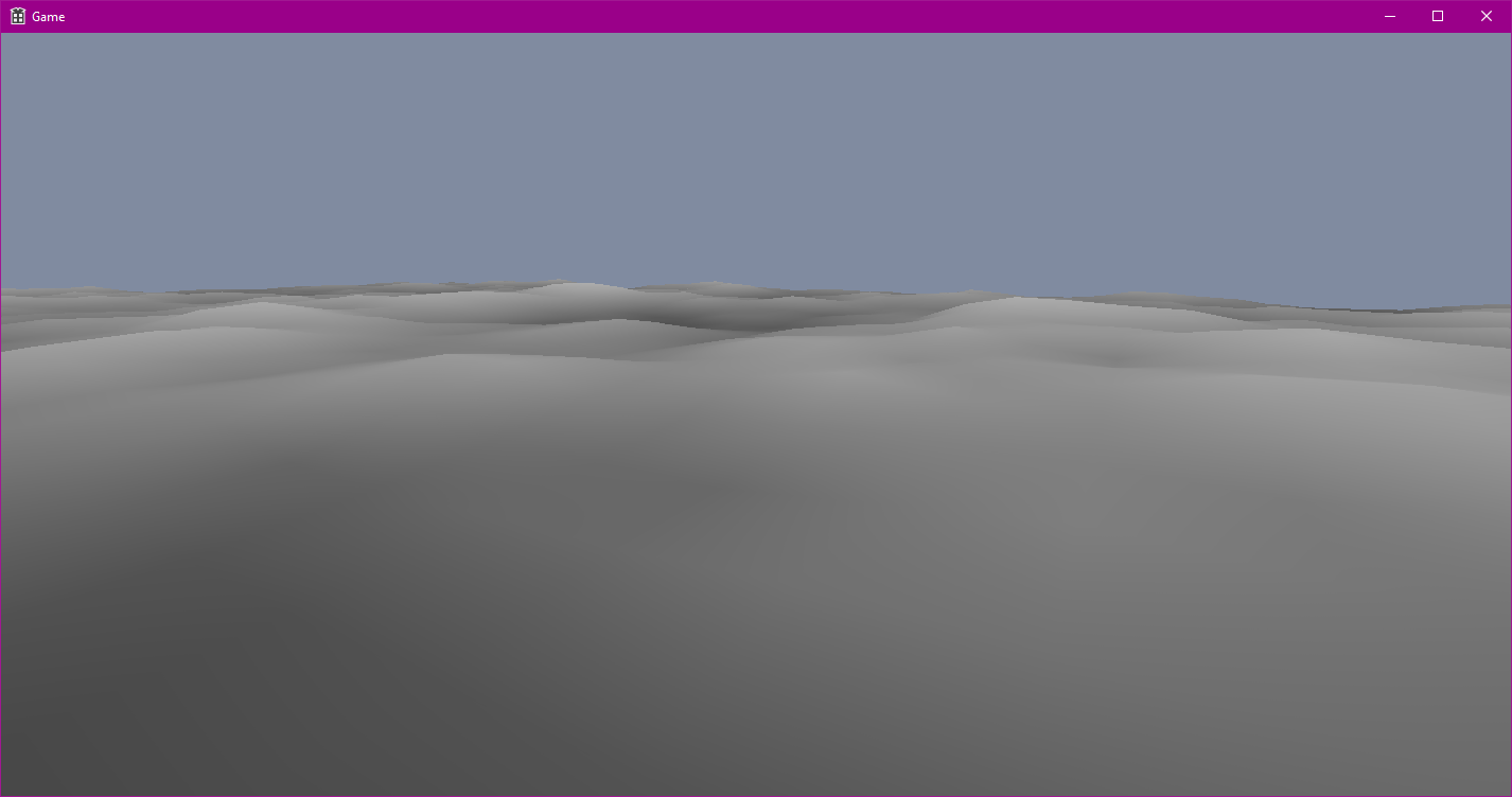
One of the larger features I implemented was a terrain generation system. The final implementation utilised a series of optimisation techniques to ensure it was fast and efficient. For example, it used a chunk based generation system which worked inline with a spatial grid as well as an instanced draw call to reduce CPU and GPU load respectively.
By utilising instancing for each chunk, I can reuse the index and vertex buffer and render the entire terrain using a single pipeline and draw call. I generate a singular flat plane of triangles to use as my base model, passing an array of height values to the vertex shader to apply the height changes on the GPU. These instances are created when the camera enters a grid node for the first time. This means that the terrain generation does not stall the engine at startup as it is only generated when it is required. Given that the initial plane is already instantiated, the only generation per chunk is the height data which consists of 64 height samples. This number can be redefined in the header and is determined by the number of points within a chunk.
Physics
One of the main takeaways from this project is that physics is hard, like really hard. This book was a lifesaver and I cannot recommend it enough. In hindsight, this section probably could’ve been a post of its own.
Rigidbodies and Forces
To provide a physics-based way to control the movement of objects within a scene, I implemented a rigidbody physics system. An object whose size and shape remain unchanged by external forces is known as a rigidbody. To calculate the forces applied to an object, I utilised Euler’s laws of motion (as they are an extension upon Newton’s laws) describing a rigidbody’s movement as combined translational and rotational dynamics. These laws correlate the motion about a centre of mass with the sum of forces and torques acting upon the body. Using the euler method to integrate over a small timestep, the forces applied upon a body can be used to calculate a new position and rotation for that frame.
My implementation for this is as follows:
void Rigidbody::Update(const float& deltaTime)
{
  if (IsEnabled == false || IsStatic() == true)
	return;

  //Compute forces and apply forces.
  //Currently, the only automatically
  //applied force is Gravity.
  if (m_IsGravityEnabled)
  {
	m_ForceSum += PHYSICS_GRAVITY_FORCE * m_Mass;
  }

  //Integrate Accelerations.
  m_Acceleration += m_ForceSum * m_InverseMass;
  m_AngularAcceleration += m_TorqueSum * m_WorldInverseTensor;

  //Integrate Velocities
  m_Velocity += m_Acceleration * deltaTime;
  m_AngularVelocity += m_AngularAcceleration * deltaTime;

  //Apply Damping
  m_Velocity *= RIGIDBODY_DAMPING_VALUE;
  m_AngularVelocity *= RIGIDBODY_DAMPING_VALUE;

  //Clear any tiny velocities to avoid jittering.
  if (m_Velocity.length() < FLT_EPSILON)
  {
	m_Velocity = glm::vec3(0.0f);
  }

  if (m_AngularVelocity.length() < FLT_EPSILON)
  {
     m_AngularVelocity = glm::vec3(0.0f);
  }

  //Apply velocities to update transform.
  m_Transform.Translate(m_Velocity * deltaTime);
  m_Transform.Rotate(m_AngularVelocity * deltaTime);

  //Recalculate Inverse Tensor based on new positions.
  m_WorldInverseTensor = m_LocalInverseTensor * glm::mat3(m_Transform.GetModelMatrix());

  //Reset per-frame forces
  m_TorqueSum = glm::vec3(0.0f);
  m_ForceSum = glm::vec3(0.0f);
}
Collision Detection
The collision detection system uses the Gilbert-Johnson-Keerthi (GJK) algorithm to determine collisions between convex colliders. It is explicitly convex colliders as GJK works under the assumption that the convex hull is the subset of something known as the Minkowski Difference. This is the set of the vector differences between all the points within two subsets.

The polygon created using the Minkowski difference represents the distance of the object relative to an origin. If the polygon contains the origin, there is an overlap between the two objects. A point exists within both polygon A and B with no difference in position, meaning they are on top of each other. This forms the basis of GJK.
Alongside this, GJK makes use of a function known as the ‘support function’. This function fetches the furthest vertex in a given direction. My implemenation for this function for an AABB collider is as follows:
glm::vec3 AABBCollider::GetFurthestPoint(const glm::vec3& direction) const
{
    glm::vec3 maxPoint = m_Corners[0];
    float maxDistance = -FLT_MAX;

    for (int i = 0; i < 8; i++)
    {
        float distance = glm::dot(m_Corners[i], direction);
        if (distance >= maxDistance)
        {
            maxDistance = distance;
            maxPoint = m_Corners[i];
        }
    }

    return maxPoint;
}
The algorithm calculates support vertices of the Minkowski polygon using the support vertices of each collider in a given direction rather than calculating the entire Minkowski polygon each frame. This reduces the number of calculations that are needed as the function may never use the majority of the polygon points. As discussed earlier, a collision only occurs when the origin is contained by the Minkowski difference polygon. To figure out when this is true, a simpler structure is needed to surround the origin. For GJK, there are Simplexes.
Determining the Simplex
A Simplex is a geometric term for the simplest possible polytope within a given dimension k; expressed as a shape containing k + 1 vertices. In 2D, this shape is a triangle and in 3D, a tetrahedron. These are used as they are much simpler to calculate whether it contains the origin. The goal is to determine the simplex that does this using the points from the Minkowski difference polygon. The process of continually testing and updating the simplex is known as ‘evolving the simplex’. For this explaination, we will only use 2D collisions to determine a triangle simplex.
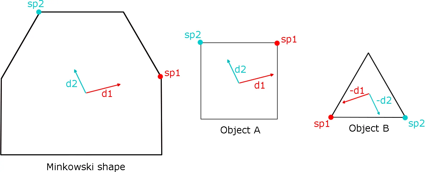
To determine an initial simplex to test, some vertices are required. The first direction to be searched can be arbitrary but for a faster result the direction of seperation between the two colliders is typically used. Using the support vertex function, the furthest vertex on the Minkowski polygon is determined as the difference between the support vertex of A taken in the given irection from the support vertex of B in the opposite direction. With the support vertex calculated using the first direction (direction of seperation), the first vertex of our simplex can be determined. The second vertex can be created from the support vertex in the opposite direction to that of the seperation. The third vertex for our 2D simplex requires a third direction that would form a triangle within the Minkowski polygon. A third direction can be determined using the original two by calculating the vector perpendicular to the vector between our initial two vertices. Having calculated these three support vertices, a triangle can be determined within the Minkowski polygon.
Evolving the Simplex
Our simplex contains the origin if it is on the ‘inside’ of all three line segments forming the shape. If the origin is ‘outside’ of any simplex, the triangle doesn’t contain it so we can return early and evolve the simplex.
Only two tests are needed when determining the origin as one is implicity done when selecting the vertices forming the simplex. By viewing the simplex as a triangle of points A, B and C, it becomes easier to visualise the actions to take.

Forming lines AB and AC provide us with directions to test for the origin. With a vector from A to the Origin, a direction perpendicular to AB and AC can be generated and using the dot product, can be checked if they are in the same direction. If each edge direction is in the same direction as the origin, the origin is within the triangle. If any edge direction is NOT in line with the vector the origin, then the origin is not within the triangle. In this case, the vertex not used to determine the edge can be discarded (case AB discards C, AC discards C) and replaced with a new support vertex in the direction provided perpendicular to the edge. This discarding and replacement of vertices is known as evolving the simplex. This continues until the triangle contains the origin but what if there is no collision? To determine this, when adding the replacement vertex there is a check as to whether the new support vertex goes past the origin. If the dot product of the vector from the new vertex to the origin and the test direction is greater than zero, then it goes past the origin.

For a more detailed explaination of the algorithm, be sure to check out Casey Muratori’s video on GJK as well as Kenton Hamaluik’s blog on Building a Collision Engine
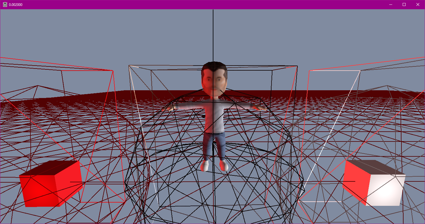
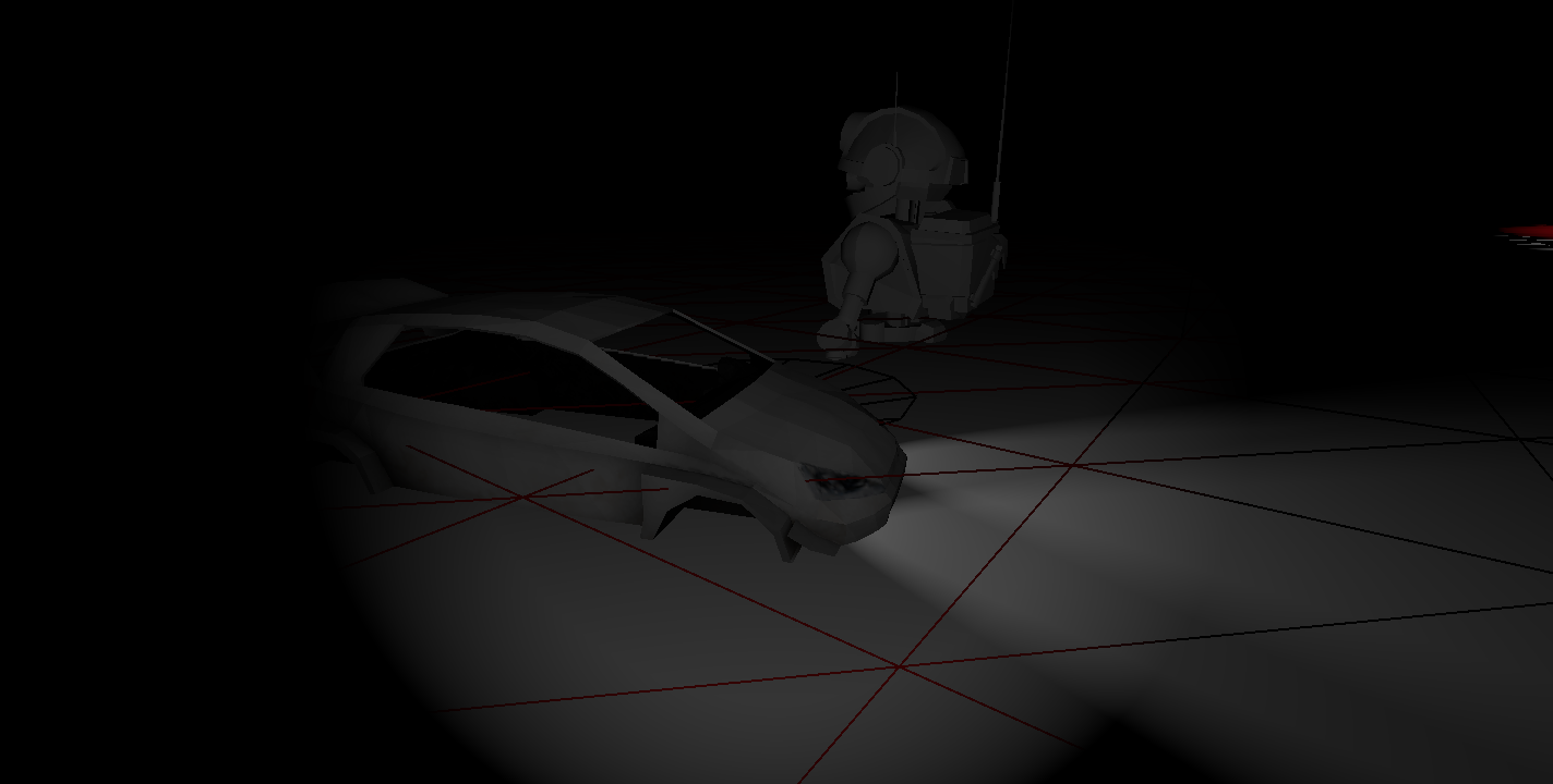
Below is an example of how collision checks are used and can be performed outside of the physics scene. This could be used in many situations as Collision::CheckCollision checks for any collider nullptrs itself. As well as this, the collision manifold is optional - passing a nullptr will avoid the EPA algorithm when the collision details are not required.
BActor* CubeA = GetWorld().GetActor("CubeA");
BActor* CubeB = GetWorld().GetActor("CubeB");

CollisionDetails manifold;

if (Collision::CheckCollision(*CubeA->GetPhysicsCollider(), *CubeB->GetPhysicsCollider(), &manifold))
{
    for (size_t i = 0; i < 2; i++)
    {
        glm::vec3 normal = manifold.CollisionPoints[i].Normal;
        glm::vec3 point = manifold.CollisionPoints[i].HitPoint;
        ServiceLocator::GetRenderer().DrawDebugLine(point, point + (normal * manifold.Depth), colours[i]);
    }
}
Optimisations
A large number of objects within a physics scene causes a large number of collision checks as every body checks against every other body. I implemented a number of common optimisation techniques to reduce this number. When creating an entity using World::CreateEntity(), if the entity requires a collider or rigidbody then it is registered with the PhysicsScene class object within the world. This ensures that only the appropriate objects are checked for collisions each tick. To further reduce the number of collision checks required, I implemented an Octree. An octree is a tree-like data structure used to divide 3D space in which each internal node can split into eight smaller nodes. I use this to split up my scene based on the number of entities surrounding an area, reducing the number of checks required per entity as they no longer need to check against objects outside of their node. The octree root exists within the PhysicsScene class and every new physics object is added directly to it. It is constructed recursively each frame, and each node able to hold 4 physics objects before splitting further.